Lecture 8. Suffix trees for NLP — различия между версиями
Polidson (обсуждение | вклад) (→Annotated suffix tree construction) |
Katya (обсуждение | вклад) |
||
| (не показаны 23 промежуточные версии ещё одного участника) | |||
| Строка 1: | Строка 1: | ||
| + | Ekaterina Chernyak, Dmitry Ilvovsky | ||
| + | |||
== Text (collection) representation model == | == Text (collection) representation model == | ||
| Строка 61: | Строка 63: | ||
Language Model [Ponte, Croft, 1998]: a probability distribution over sequences of words. | Language Model [Ponte, Croft, 1998]: a probability distribution over sequences of words. | ||
| − | Unigram model: p(t | + | Unigram model: p(t<sub>1</sub> t<sub>2</sub> t<sub>3</sub> ) = p(t<sub>1</sub>)p(t<sub>2</sub>)p(t<sub>3</sub>) |
| − | Bigram model: p(t < | + | Bigram model: p(t<sub>1</sub> t<sub>2</sub> t<sub>3</sub>) = p(t<sub>1</sub>|BOS) p(t<sub>2</sub>|t<sub>1</sub>)p(t<sub>3</sub>|t<sub>2</sub>)p(EOS|t<sub>3</sub>) |
[[Файл:L8 1.jpg|слева]] | [[Файл:L8 1.jpg|слева]] | ||
| Строка 108: | Строка 110: | ||
* Feature generation for text classification [Zhang, Lee, 2006] | * Feature generation for text classification [Zhang, Lee, 2006] | ||
| − | [[Файл:L8 2.jpg|Suffix tree: Example from [Gus�led, 1998]]] | + | [[Файл:L8 2.jpg|350px|Suffix tree: Example from [Gus�led, 1998]]] |
== Annotated suffix tree == | == Annotated suffix tree == | ||
| Строка 118: | Строка 120: | ||
* Every node is labeled by the frequency of the text fragment encoded by the path from the root to the node. | * Every node is labeled by the frequency of the text fragment encoded by the path from the root to the node. | ||
| − | [[Файл:L8 3.jpg]] | + | [[Файл:L8 3.jpg|350px]] |
=== Annotated suffix tree construction === | === Annotated suffix tree construction === | ||
| Строка 130: | Строка 132: | ||
* Add "G" as a single node with frequency equal to unity. | * Add "G" as a single node with frequency equal to unity. | ||
| − | [[Файл:L8 4.jpg]] | + | [[Файл:L8 4.jpg|350px]] |
Using Naive algorithm we add the second string "DINING". Complexity: both O(n^2) time and space, where n is the number of input strings. Frequency of the root node is the sum of the first level node frequencies. | Using Naive algorithm we add the second string "DINING". Complexity: both O(n^2) time and space, where n is the number of input strings. Frequency of the root node is the sum of the first level node frequencies. | ||
| Строка 136: | Строка 138: | ||
=== Annotated suffix tree scoring === | === Annotated suffix tree scoring === | ||
| − | [[Файл:L8 5.jpg|слева]] | + | [[Файл:L8 5.jpg|550px|слева]] |
| − | [[Файл:L8 6.jpg|слева]] | + | [[Файл:L8 6.jpg|550px|слева]] |
| − | <br> <br> <br> <br> <br> <br> <br> <br> <br> <br> <br> <br> <br> <br> <br> <br> <br> <br> <br> <br> <br> <br> <br> <br> <br> <br> <br> <br> | + | <br> <br> <br> <br> <br> <br> <br> <br> <br> <br> <br> <br> <br> <br> <br> <br> <br> <br> <br> <br> <br> <br> <br> <br> <br> <br> <br> <br> <br> <br> <br> |
=== Applications of AST === | === Applications of AST === | ||
| Строка 185: | Строка 187: | ||
[[Файл:L8 7.jpg]] | [[Файл:L8 7.jpg]] | ||
| − | |||
| − | |||
| − | |||
== Taxonomy refinement == | == Taxonomy refinement == | ||
| Строка 194: | Строка 193: | ||
Still we have something in educational standards. We can use Wikipedia to refine it. | Still we have something in educational standards. We can use Wikipedia to refine it. | ||
| − | [[Файл:L8 8.jpg|слева]] | + | [[Файл:L8 8.jpg|400px|слева]] |
| − | [[Файл:L8 9.jpg|слева]] | + | [[Файл:L8 9.jpg|400px|слева]] |
| − | [[Файл:L8 10.jpg|слева|The refining scheme. Initial taxonomy topics are in rectangles, the Wikipedia categories and subcategories are in rounded rectangles, the Wikipedia articles are in the ovals, and the leaf descriptors are in the clouds.]] | + | [[Файл:L8 10.jpg|600px|слева|The refining scheme. Initial taxonomy topics are in rectangles, the Wikipedia categories and subcategories are in rounded rectangles, the Wikipedia articles are in the ovals, and the leaf descriptors are in the clouds.]] |
| − | <br> <br> <br> <br> <br> <br> <br> <br> <br> <br> <br> <br> <br> <br> <br> <br> <br> <br> <br> <br> <br> <br> <br> <br> <br> <br> <br> <br> <br> <br> <br> <br> <br> <br> <br> <br> <br> | + | <br> <br> <br> <br> <br> <br> <br> <br> <br> <br> <br> <br> <br> <br> <br> <br> <br> <br> <br> <br> <br> <br> <br> <br> <br> <br> <br> |
| + | <br> <br> <br> <br> <br> <br> <br> <br> <br> <br> | ||
# Specify the domain of taxonomy to be refined and set the frame of taxonomy manually. | # Specify the domain of taxonomy to be refined and set the frame of taxonomy manually. | ||
# Download, from the Wikipedia, the category tree and articles from the domain under consideration. | # Download, from the Wikipedia, the category tree and articles from the domain under consideration. | ||
| Строка 208: | Строка 208: | ||
# Extract relevant keywords from Wikipedia articles and use them as leaf descriptors. | # Extract relevant keywords from Wikipedia articles and use them as leaf descriptors. | ||
| − | |||
| − | |||
| − | |||
| − | <br> <br> <br> <br> <br> <br> <br> <br> <br> <br> <br> <br> <br> <br> <br> <br> <br> <br> <br> <br> <br> <br> <br> <br> <br> <br> <br> <br> <br> <br> <br> <br> <br> <br> <br> <br> <br> <br> <br> <br> <br> <br> <br> <br> <br> <br> <br> <br> <br> <br> <br> <br> | + | [[Файл:L8 11.jpg|500px|слева]] |
| + | [[Файл:L8 12.jpg|600px|слева|The fragment of refined PTMS taxonomy. Lower layers are shown.]] | ||
| + | [[Файл:L8 13.jpg|600px|слева|The fragment of refined PTMS taxonomy. Lower layers are shown.]] | ||
| + | |||
| + | <br> <br> <br> <br> <br> <br> <br> <br> <br> <br> <br> <br> <br> <br> <br> <br> <br> <br> <br> <br> <br> <br> <br> <br> <br> <br> <br> <br> <br> <br> <br> <br> <br> <br> <br> <br> <br> <br> <br> <br> <br> | ||
| + | <br> <br> <br> <br> <br> <br> <br> <br> <br> <br> <br> <br> <br> | ||
== German compound splitting == | == German compound splitting == | ||
| Строка 231: | Строка 233: | ||
== Reference graph == | == Reference graph == | ||
| + | |||
| + | [[Файл:L8 14.jpg|450px|слева]] | ||
| + | |||
| + | <br> <br> <br> <br> <br> <br> | ||
| + | Reference graph is a graph of association rules. Not interesting itself, but: | ||
| + | * Dynamics | ||
| + | * Link analysis | ||
| + | * Visualization with different options | ||
| + | * Data: Russian newspapers | ||
| + | * Nodes: Key words and phrases | ||
| + | * Edges: A ⇒ B: the key word or phrase B occurs with a higher probability if the key word or phrase A occurs in the same text Features: Easy extension to temporal case and possibility of well developed graph analysis methods | ||
| + | |||
| + | Reference graphs can be used as a tool of information discovery and search and as a tool for temporal analysis. | ||
| + | |||
| + | [[Файл:L8 15.jpg|слева]] | ||
| + | |||
| + | <br> <br> <br> <br> <br> <br> <br> <br> <br> <br> <br> <br> <br> <br> <br> <br> <br> | ||
== Profound filtering == | == Profound filtering == | ||
| + | |||
| + | Za-***-t' | ||
| + | |||
| + | Pro-***-t' | ||
| + | |||
| + | Vy-***-t' | ||
| + | |||
| + | Na-***-t' | ||
| + | |||
| + | There are dictionaries of *** , but new words appear. And we have new policy of using profanity in the Web. Also stemming fails since it does not strip preffixes. | ||
| + | |||
| + | '''Idea''': Get a text from the web. Construct an AST from it and index. | ||
| + | Score *** to it. Find profound words. | ||
| + | Chernyak, | ||
== Implementation == | == Implementation == | ||
| + | |||
| + | AST construction and scoring in linear time and space using suffix arrays is developed by Mikhail Dubov. Take a look at his library for Python at GitHub: [https://github.com/msdubov/AST-text-analysis]. By the way, there is a huge theory about suffix trees and string algorithms I did not talk today about. | ||
Текущая версия на 22:49, 5 ноября 2016
Ekaterina Chernyak, Dmitry Ilvovsky
Содержание
Text (collection) representation model
Vector Space Models
Vector Space Models, VSM [Salton, Wong, Yang, 1975] : every text is a vector in a space of terms. Usually is used along with cosine similarity measure.
Pro:
- Makes linear algebra operation and thus machine learning applicable
- Is simple and based on human intuition
Contra:
- The more the words are there in the the text, the higher is the cosinesimilarity
- Word order is lost
- Need some additional hacks to use bigrams and ngrams as terms
Applications:
- Information retrieval
- Topic, genre and maybe sentiment classification
- Extractive summarization
- Spam filtering
Generalized Vector Space Models
Generalized Vector Space Models, GVSM [Wong, Ziarko, Wong, 1985]: introduces a term to term correlation in the VSM.
Pro:
- Is still easy
- Synonyms or near synonyms are introduced into the model
- Term to term correlation may be computed in several ways: co-occurrences in the collection under consideration, co-occurrences in a large corpus, thesaurus-based relations
Contra:
- A lot of computations: if jVj = n (the number of terms), there are 2ndimensions in the GVSM
- Word order is lost
- Need some additional hacks to use bigrams and ngrams as terms
Applications: mainly information retrieval
Vector Space Model of Semantics
Vector Space Model of Semantics [Turney, Pantel, 2010]: terms are vector in the space of contexts (usually, also terms).
Pro:
- Is still easy
- Allows to find semantically similar words
- Very loved by scientific community
Contra:
- Word order is lost
- Need some additional hacks to use bigrams and ngrams as terms
Applications:
- Word similarity detection, clustering, classification
- Automatic thesaurus generation
- Word sense disambiguation
- Context-sensitive spelling correction
- Textual advertising
Language Model [Ponte, Croft, 1998]
Language Model [Ponte, Croft, 1998]: a probability distribution over sequences of words.
Unigram model: p(t1 t2 t3 ) = p(t1)p(t2)p(t3)
Bigram model: p(t1 t2 t3) = p(t1|BOS) p(t2|t1)p(t3|t2)p(EOS|t3)
Language Model [Ponte, Croft, 1998]: a probability distribution over sequences of words.
Pro:
- The word order is not lost
- Makes Markov chain theory applicable
Contra:
- The problem of unseen words
- How to choose n?
- Long relations between words or sentences (for example, anaphora) are lost
Applications:
- Information retrieval
- Text generation
- Abstractive summarization
- Speech recognition
- Speech generation
To sum up:
- VSM-like models: no word order, algebraic structures, classification of any kind, stemming and lemmatization for dimension reduction
- LM-like models: partially word order, Markov chains, generation of text and speech
- What if new word appears? What if there is a typo? What if stemming is not always correct? Use edit distance on words or stems or use symbol ngrams instead as terms or ...
Suffix tree
Annotated suffix tree (AST)
The suffix tree is a data structure used for storing of and searching for strings of characters and their fragments.
Suffix trees in NLP:
- Text clustering [Zamir, Etzioni,1998]
- Language model for MT [Kennington et al., 2012] and IR [Huang, Powers, 2008]
- Feature generation for text classification [Zhang, Lee, 2006]
Annotated suffix tree
Annotated suffix tree (AST) [Pampapathi, Mirkin, Levene, 2006]:
An annotated suffix tree is a data structure used for computing and storing all fragments of the text and their frequencies. It is a rooted tree in which:
- Every node corresponds to one character
- Every node is labeled by the frequency of the text fragment encoded by the path from the root to the node.
Annotated suffix tree construction
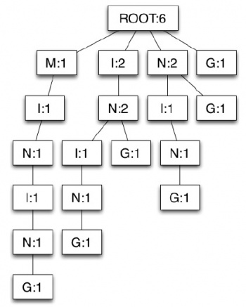
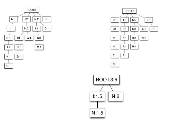
"MINING" has 6 suffixes: "MINING", "INING", "NING", "ING", "NG", "G"
Naive algorithm for AST construction
- Start with "MINING", add it as a chain of nodes with frequencies equal to unity. Add "INING" and "NING" the same way.
- When adding "ING", note that there is already a path from root that encodes / reads "I N". Increase the frequencies in this path by 1. Add "G" to the end of the path. When adding "NG", note "G" and react in the same way.
- Add "G" as a single node with frequency equal to unity.
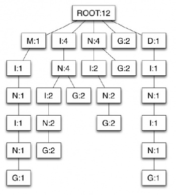
Using Naive algorithm we add the second string "DINING". Complexity: both O(n^2) time and space, where n is the number of input strings. Frequency of the root node is the sum of the first level node frequencies.
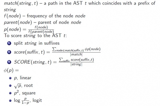
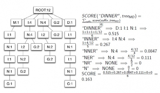
Annotated suffix tree scoring
Applications of AST
- Spam filtering [Pampapathi, Mirkin, Levene, 2006]
- Text categorization and clustering [Chernyak, Chugunova, Mirkin, 2010]
- Text summarization [Yakovlev, Chernyak, 2014]
- Taxonomy refinement [Chernyak, Mirkin, 2013]
- German compound splitting [Provatorova, Chernyak, 201x]
- AST as a string kernel [Dubov, 201x]
- Reference graph construction [Dubov, Chernyak, Mirkin, 201x]
- Profound filtering
- Duplicate detection
Spam filtering
- Construct two huge ASTs: spam AST and ham AST
- Introduce match permutation (swaping symbols in the match) to SCORE
- Test versus Naive Bayes classifier on a standart datasets (The Ling-Spam corpus, Spam Assassin public corpus, The BBKSpam04 corpus)
- Beat it (in terms of spam precision and spam recall)!
Unsupervised text categorization
Input 1: 5k+ abstracts from ACM journal and ACM CCS (English). Every abstract is annotated with some of the ACM CCS topics.
Input 2: 100k+ web page description from Yandex Categories (YaCa) and Yandex Categories (Russian). Every description belongs to a YaCa categories.
Note: We know right answers! We try to reproduce them computationally. Pure scientific joy. No business applications.
Task: different models of text collection representation, relevance measures and AST scoring ⇒ relevance() Score relevance(taxonomy topic) and relevance(YaCa category) to abstracts and descriptions. Score the taxonomy topics and YaCa categories in descending order. Calculate how many right answers are there. Use nDCG and MAP to evaluate the quality.
Text summarization
TextRank is an efficient algorithm for extractive text summarization. Let us construct graph, where nodes stand for single sentences and edges connect sequential sentences. Than we can use the VSM and cosine similarity to compute the similarity between sentences and run PageRank to get the most important sentences. Let us replace the cosine similarity with scoring common AST.
A common AST of two ASTs is a tree, that consists of all chains of nodes that coincide in the ASTs. The frequencies are computed as average. Scoring the common AST (i.e.scoring all the paths in the tree according to SCORE) suits as sentence similarity measure.
Input 1: DUC 2004 (a text collection for text summarization)
Input 2: home made collection of gazeta.ru papers.
Quality measures: precision
Taxonomy refinement
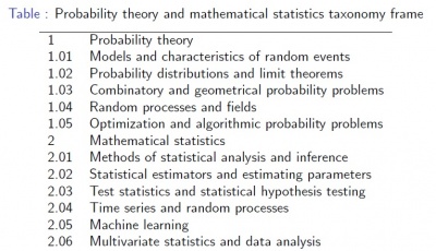
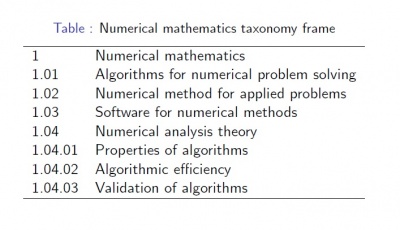
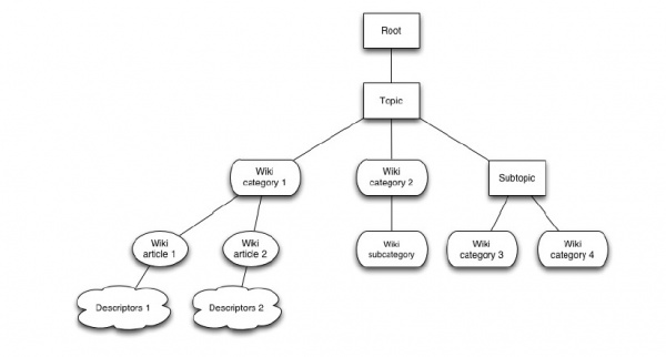
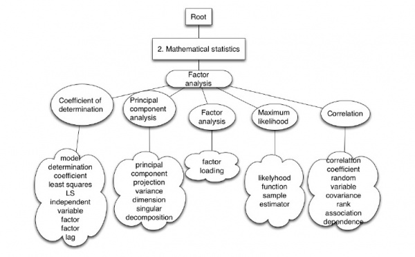
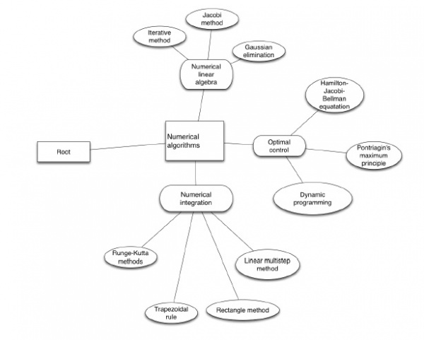
No taxonomy of mathematics in Russian! Let us construct one. Still we have something in educational standards. We can use Wikipedia to refine it.
- Specify the domain of taxonomy to be refined and set the frame of taxonomy manually.
- Download, from the Wikipedia, the category tree and articles from the domain under consideration.
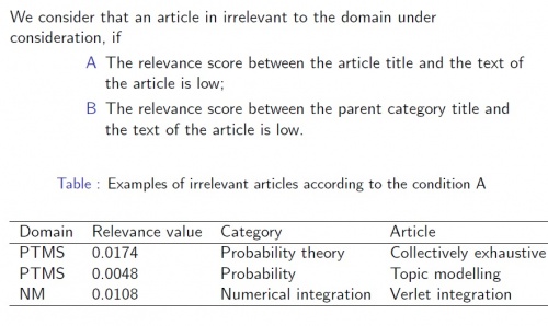
- Clean the category subtree of irrelevant articles.
- Clean the category subtree of irrelevant subcategories.
- Assign the remaining Wikipedia categories to the taxonomy topics.
- Form the intermediate layers of the taxonomy
- Use Wikipedia articles in each of the added category nodes as its leaves.
- Extract relevant keywords from Wikipedia articles and use them as leaf descriptors.
German compound splitting
Liebeskummer — heart-sickness — Lieb-es-kumm-er Bilderrahmen — picture frame — Bild-er-rahm-en Schmerzensgeld — compensation — Schmerz-ens-geld Gedankenfreiheit — freedom of thought — Gedank-en-frei-heit Schweineeisch — pork — Schwein-e-eisch Trinkgeld — tip — Trink-geld
To split a compound:
- write complex linguistics rules
- use machine learning algorithms
- (hypothesis) construct an AST from a list of simple words, than score compounds to this tree
It is a problem to find a list of German words that does not contain compounds.
Reference graph
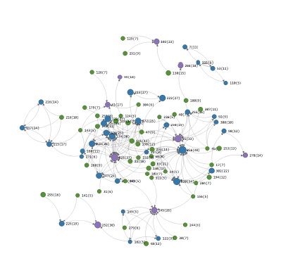
Reference graph is a graph of association rules. Not interesting itself, but:
- Dynamics
- Link analysis
- Visualization with different options
- Data: Russian newspapers
- Nodes: Key words and phrases
- Edges: A ⇒ B: the key word or phrase B occurs with a higher probability if the key word or phrase A occurs in the same text Features: Easy extension to temporal case and possibility of well developed graph analysis methods
Reference graphs can be used as a tool of information discovery and search and as a tool for temporal analysis.
Profound filtering
Za-***-t'
Pro-***-t'
Vy-***-t'
Na-***-t'
There are dictionaries of *** , but new words appear. And we have new policy of using profanity in the Web. Also stemming fails since it does not strip preffixes.
Idea: Get a text from the web. Construct an AST from it and index. Score *** to it. Find profound words. Chernyak,
Implementation
AST construction and scoring in linear time and space using suffix arrays is developed by Mikhail Dubov. Take a look at his library for Python at GitHub: [1]. By the way, there is a huge theory about suffix trees and string algorithms I did not talk today about.

![Suffix tree: Example from [Gus�led, 1998]](/images/thumb/c/c6/L8_2.jpg/350px-L8_2.jpg)
